It has been known for almost three decades that the solar corona is comprised of closed loops. Despite vast theoretical efforts, it seems to be a long way before we feel we understand the mechanism by which these loops are heated to coronal temperatures. One thing that complicates comparisons between theory and observed data may be the presence of loops of different temperatures ranging 0.5-10 MK, even ignoring hotter loops created in major flares. No single instrument to date is sensitive to all these temperatures. For example, the plot below (click to enlarge) shows that SXT, a grazing-incidence telescope, is sensitive to a broad temperature range, but that its sensitivity drops dramatically below 2-6 MK depending on the filter. In contrast, TRACE, with normal-incidence optics, has more peaked sensitivities toward lower temperatures.
Also, the spatial resolution of TRACE is five times as good as that of SXT.
As a result, the images of these two instruments look quite different. In SXT images, coronal loops are hard to define. This should be attributable to the difference of spatial resolution, and the broad temperature sensitivity of SXT (picking up plasmas of different temperatures along the line of sight), but another reason may be that hot loops are intrinsically diffuse. The left figure below (click to enlarge) shows an SXT image of an active region. Some of what appear to be loops are traced in the right figure.
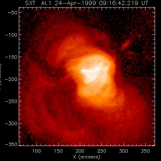
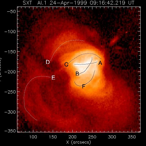
In order to identify a loop, we first need to spot the footpoints, but it is not simple, since they are cooler than what SXT can see. Bright features A and B are probably loops, although footpoints on the right side are not 100 % certain. Others are less trivial. In addition, there is a structure to the southwest, but it lacks discrete loop-like patterns. Various filters in the image processing package were applied to bring up the loops, but without success.
These traced loops are overplotted on nearly simultaneous TRACE images as in the following figures (click to enlarge). They are (from left to right) at 284 Ĺ, 195 Ĺ and 171 Ĺ.
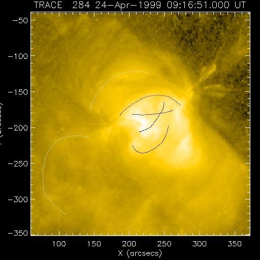
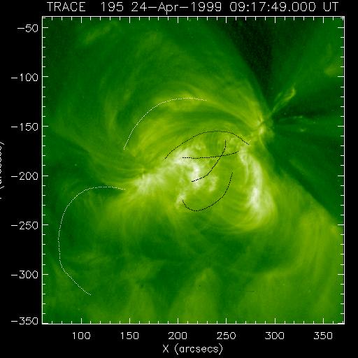
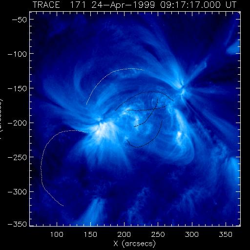
Even in the image at 284 Ĺ, where the temperature response somewhat overlaps with that of SXT, we do not clearly see the loops, despite the overall similarity of bright areas. If the TRACE images reveal the base of the loops. identification of the footpoints do not look correct for loops D, E and F. This difficulty of identifying the base of SXT loops prevents us from obtaining their geometry-deconvolved plasma parameters (see Aschwanden et al. (1999) for EUV loops).
Concerning the base of loops, Peres et al. (1994) first argued, on the basis of NIXT and SXT data, that the low-lying features reminiscent of H-alpha plages are due to high-pressure loops. Recently, Berger et al. (1999) and Fletcher and de Pontiue (1999) found similar features, better resolved in TRACE images (notably at 171 Ĺ), and called them ``moss'', a nomenclature not easily understandable to non-native English speakers. In terms of physics, it is reasonable to consider the moss to be due to heat conduction from hot loops (see a previous nugget). But observationally, it is not always straightforward to locate the moss at the base of SXT loops, which tend to be diffuse. For example, in the 171 Ĺ image shown above, there are mossy areas in the south (say, 200 < x < 330, -350 < y <-300), but whose footpoints are these? Maybe some diffuse loops, which may not have as high pressure as to produce enhaned emission at the base. If that is the case, the moss can be used to locate the base of these diffuse loops, as suggested by Peres et al. (1994) for locating high-pressure loops.
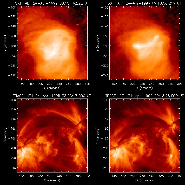
In the central part of this active region, bright loops appeared and disappeared in SXT images. They were small flares or tansient brightenings, and it is likely that any bright loops in an active region formed in this way. These loops must be dense, so they should contribute to the moss. However, the following figure (click to enlarge) suggests that the moss did not change much around the time a bright loop appeared (between 08:55 and 09:16). Of course we need quantitative analysis to find out how much the new bright loops affect the underlying moss. In this central active region, even areas between the ends of bright loops are mossy.
Lastly, I tried to find traces of bright loops in TRACE images before and after they become visible in SXT images. But I could not find them. This suggests that hot (> 3 MK) loops do not start from cooler (~1 MK) loops. When loops are even cooler, say 0.5 MK, some of them get bigger energies than others and become SXT loops and others smaller energies to become TRACE/EIT loops. Further action items include finding how the cooler loops compare with the scaling law derived for hot stationary loops. According to the above scaling law, a 4.5 MK loop has to be 9 times as dense as a 1.5 MK loop with the same length. But this kind of discussion may not be so easy, since the loop length depends on geometry and the effect of different structures along the line of sight is not obvious for TRACE loops, even acknowledging the professional work of dynamic streoscopy by Aschwanden et al. (1999).
19 September 1999: Nariaki Nitta (nitta@lmsal.com)