Often an interesting "discovery" turns out to be due to mis-use or too naive use of data. The temperature information from SXT data is certainly important, telling us a lot about heating. However, before you take into account various uncertainties, it may not be a good idea to take SXT filter-ratio temperature maps at face value, especially when you discuss where in a flare intense heating takes place. Blackbox approach does not readily give you useful information.
SXT has five analysis filters which vary in the dependence of transmission on wavelength. The ratio of intensity in two of the filters is used to get temperature of the object. The underlying assumption in this exercise is that the object is isothermal, i.e., it has only one temperature, which is clearly too over-simplifying for solar corona. But the SXT "color" or filter-ratio temperature is still a measure of real plasma temperature, which may be obtained only by spectral line diagnostics.
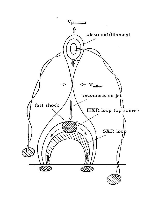
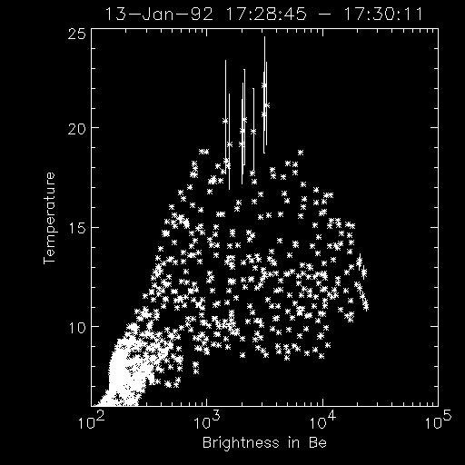
SXT is great in following dynamic phenomena in the solar corona, frequent brightenings here and there. The images are so beautiful. But we should remember that a brightening can be due to an increase in density, rather than temperature, meaning that bright areas in SXT images do not necessarily represent locations of heating. For flares, it has become almost a consensus (at least at a cartoon level) to locate the energy release region outside or above the magnetic loop bright in soft X-rays. An example is this. More cartoons like this for flares and CMEs are available here. So we need to deal with the temperature distribution, by taking the ratio of a pair of images in different filters. This "filter ratio technique" has been (at least to this author) as challenging as analyzing data from other Yohkoh instruments such as HXT and BCS. First, even though a flare is a bright object in X-rays, detection of high-temperature areas is limited by count statistics, because such areas tend to occur where the intensity is much less than the brightest pixel. Indeed, the following scatter plot (click to enlarge) shows that high-temperature pixels tend to have low brightness. The temperature in this plot, as in other figures in this nugget, comes from the ratio between thick Al and Be filters.
This plot also shows that the error bars (due to count statistics) for the temperature of these hot pixels are quite large, even after we sum up 6 or 7 images to improve the signal-to-noise ratio. The following plot (click to enlarge) compares the error bars of temperature maps, when we use a single image pair (left) and a summed image pair (right). The top and middle panels represent temperature and emission measure (density^2 x depth), respectively, and the bottom panels plot these quantities across the line indicated in the top and middle panels. We see big error bars to the temperature for a single image pair (no time integration), although the emission measure has relatively small uncertainties. For this reason, the temperature maps in this nugget reflect summation of several images in either filter before taking the ratio.

We also note an increase in temperature toward left, i.e., lower altitudes. The presence of high temperature regions lower down is not predicted in any popular cartoons that are based on magnetic reconnection. We usually attribute this temperature gradient to spurious effects coming from the fact that a point source appears slightly larger in the Be image than in the thick Al image. No conclusive work has so far been shown to this author on the characterization of the SXT point spread function (PSF) for images in these filters. It is clearly an area that needs lots of development. All I can say at the moment is that the effect of slightly different PSFs in these filters would be more pronounced for more compact sources. Judgment of the reality of high-temperature pixels is not fully objective. Often used criteria include (1) their distribution is wider than 1-2 pixels, (2) they appear consistently from one temperature map to next, (3) they occur where the intensity is not extremely low, (4) they do not show strong dependence on changes in the intensity images, etc. I know, some of these criteria are really vague.
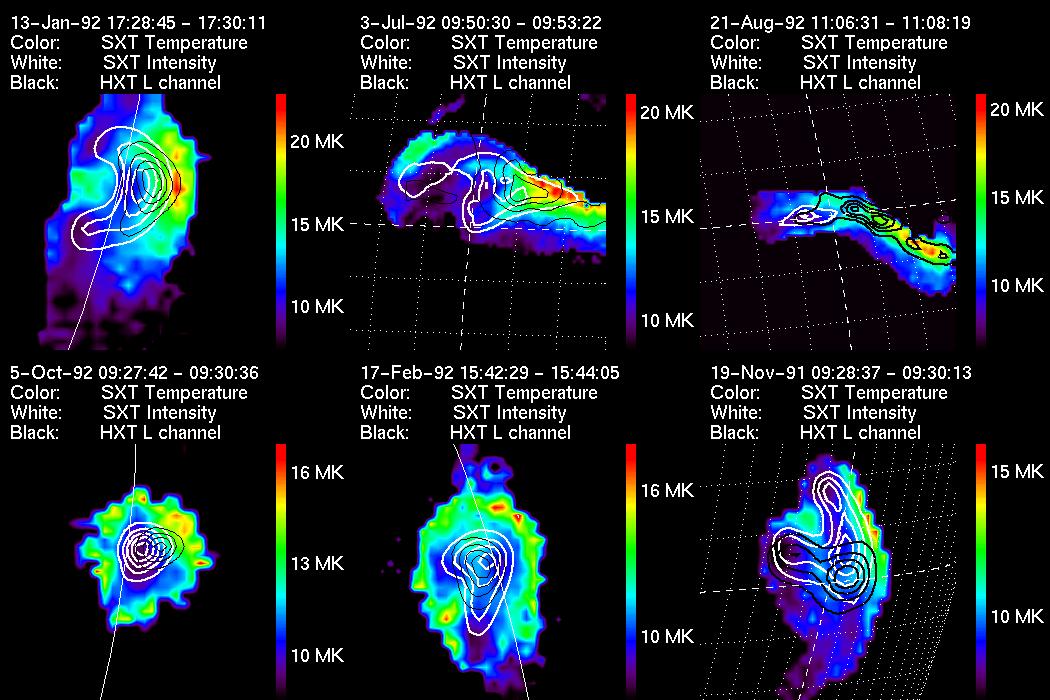
The following figure shows for 6 flares a temperature map over-plotted with the SXT intensity image and HXT L-channel (14-23 keV) image. Most of these flares have been studied by at least somebody like the prolific Aschwanden. Using the criteria given above, I believe that the high-temperature regions are captured in the upper flares, but that the lower flares are dominated by spurious effects. None of the three flares in the upper panels show that the SXT high-temperature area is exactly co-spatial with the HXT L-channel source. As I indicated above, these temperature maps do not readily provide the plasma or electron temperature of the flares, because of the broad-band nature of the SXT instrument. Another pair of filters can show different temperatures, meaning that a given line of sight is not intersected by plasma characterized by a single temperature. But judging from the offset between the SXT hot regions (in red) and the HXT L-channel sources (black contours), the former should not have much higher temperatures than given by the SXT filter ratio. This means a very hot or super-hot region (as represented by the HXT L-channel source, which is about 35 MK on the basis of the ratio between L and M1 channels) is located between the areas not as hot, as far as the flare of 13-Jan-92 is concerned. So from low to high altitudes, cool, very hot and mildly hot. I wonder how this temperature gradient is accommodated in the cartoon introduced above. We can of course assume that the HXT L-channel source comes from non-thermal electrons trapped in the corona. Then it does not have to appear hot in SXT temperature maps.
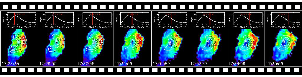
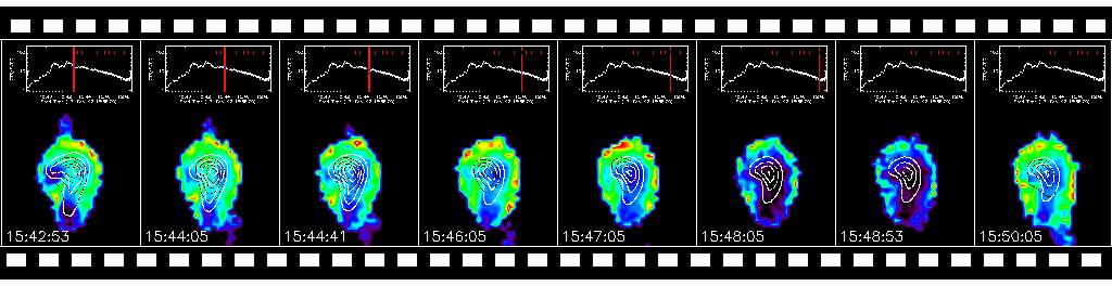
The following movies show evolution of the relation between the SXT temperature and intensity distributions and the HXT L-channel source. It appears that the above positional relation (cool, very hot, mildly hot as we go higher) is augmented toward the end of the first flare. Note that the mildly hot area becomes hottest slightly after the peak hard X-ray flux, which is shown above the images. The second flare shows that the HXT L-channel source is nearly co-spatial with the SXT intensity peak, with the SXT temperature maps dominated by the spurious edge.
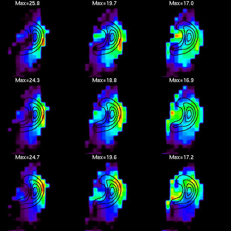
Let me comment on the possibility that the uncorrected spacecraft jitter may explain the spurious hot edges in SXT temperature maps, as proposed by a Polish team. See this page for the reference (their full paper). Indeed, as the following figure indicates, only a slight shift of one of the image pair can drastically change the appearance of the high-temperature regions. It shows SXT temperature maps for the 13 January flare, when the thick Al image is artificially shifted by 0.25 pixels in the corresponding directions -- the central map has no shift. The high-temperature region above the soft X-ray loop is enhanced in the maps in the left column, and almost vanishes in those in the right column.
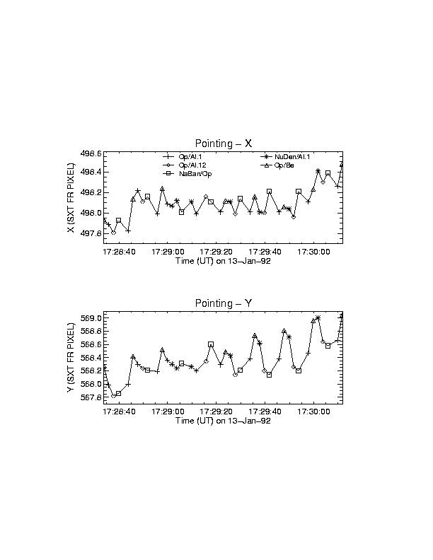
But I do not believe that this kind of artificial manipulation should be applied to SXT data. The following plot shows the spacecraft jitter as sampled at the same cadence (2 s) as the SXT images. Look for the lozenge and triangle symbols. These represent the spacecraft pointing for images in thick Al and Be filters. As far as we know, these are corrected accurately in standard analysis software. The only possibility is that the spacecraft moves a lot within 100 ms, before the SXT shutter actually opens. But Hugh Hudson indicates that this effect is negligible.
Finally, I would like to emphasize that emission measure of the high-temperature areas outside the loop is more than a order of magnitude too small to account for BCS Fe XXV observations. The SXT filter-ratio temperature may be similar to BCS in these areas, but I believe that 20 MK resides in the loop and the HXT L channel source on the basis of considerations on emission measure.