 Helioseismology
Helioseismology
Helioseismology
Helioseismology
The science studying wave oscillations in the Sun is called helioseismology. One can view the physical processes involved, in the same way that seismologists learn about the Earth's interior by monitoring waves caused by earthquakes. Temperature, composition, and motions deep in the Sun influence the oscillation periods and yield insights into conditions in the solar interior.
Waves
The primary physics in both seismology and helioseismology are wave motions that are excited in the body's (Earth or Sun) interior and that propagate through a medium. However, there are many differences in number and type of waves for both terrestrial and solar environments.For the Earth, we usually have one (or a few) source(s) of agitation: earthquake(s).
For the Sun, no one source generates solar "seismic" waves. The sources of agitation causing the solar waves that we observe are processes in the larger convective region. Because there is no one source, we can treat the sources as a continuum, so the ringing Sun is like a bell struck continually with many tiny sand grains.
On the Sun's surface, the waves appear as up and down oscillations of the gases, observed as Doppler shifts of spectrum lines. If one assumes that a typical visible solar spectrum line has a wavelength of about 600 nanometers and a width of about 10 picometers, then a velocity of 1 meter per second shifts the line about 0.002 picometers [Harvey, 1995, pp. 34]. In helioseismology, individual oscillation modes have amplitudes of no more than about 0.1 meters per second. Therefore the observational goal is to measure shifts of a spectrum line to an accuracy of parts per million of its width.
Oscillation Modes
The three different kinds of waves that helioseismologists measure or look for are: acoustic, gravity, and surface gravity waves. These three waves generate p modes, g modes, and f modes, respectively, as resonant modes of oscillation because the Sun acts as a resonant cavity. There are about 10^7 p and f modes alone. [Harvey, 1995, pp. 33]. Each oscillation mode is sampling different parts of the solar interior. The spectrum of the detected oscillations arises from modes with periods ranging from about 1.5 minutes to about 20 minutes and with horizontal wavelengths of between less then a few thousand kilometers to the length of the solar globe [Gough and Toomre, p. 627, 1991].The image below was generated by the computer to represent an acoustic wave ( p mode wave) resonating in the interior of the Sun.
The figure above shows one set of standing waves of the Sun's vibrations. Here, the radial order is n = 14, angular degree is l = 20, and the angular order is m = 16. Red and blue show element displacements of opposite sign. The frequency of this mode determined from the MDI data is 2935.88 +/- 0.2 microHz.
(You can also download a postscript version of the above figure and read the preprint, (5.7 Mb,postscript) titled: Structure and Rotation of the Solar Interior: Initial Results from the MDI Medium-L Program.)
Why does the Sun act as a resonant cavity? Acoustic waves become trapped in a region bounded on top by a large density drop near the surface, and bounded on the bottom by an increase in sound speed that refracts a downward propagating wave back toward the surface. A standing wave is created.
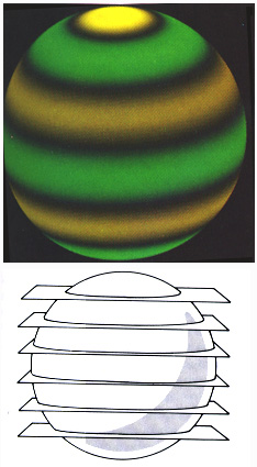
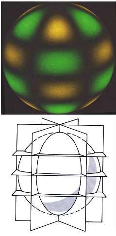
Physically and mathematically, one can understand the oscillation modes using spherical harmonics: l, and m, and n values. The spherical harmonic functions provide the nodes of standing wave patterns. The order n is the number of nodes in the radial direction. The harmonic degree, l, indicates the number of node lines on the surface, which is the total number of planes slicing through the Sun. The azimuthal number m, describes the number of planes slicing through the Sun longitudinally.
Picture credits: Noyes, Robert, "The Sun", in _The New Solar System_, J. Kelly Beatty and A. Chaikin ed., Sky Publishing Corporation, 1990, pg. 23.The figure on the left shows spherical harmonic numbers l = 6 and m = 0. The dark regions are the nodal boundaries, the green colors denote areas moving radially outward, and yellow colors show those areas moving radially inward. The figure on the right shows spherical harmonic numbers l = 6 and m = 3. The dark regions are the nodal boundaries, the green colors denote areas moving radially outward, and yellow colors show those areas moving radially inward.
We can learn about many astrophysical processes by studying the Sun as a star. We can learn about nuclear energy generation, energy flows, interaction of magnetic fields with matter, and particle acceleration to high energies. The theory of stellar structure and evolution is a principal foundation of astrophysics and of much of our current understanding of the universe. And a major goal of helioseismology is to determine if our theories of stellar structure and evolution are correct.
Solar Structure
The theories of stellar structure and evolution applied to our Sun are called solar models. The solar model equations must be solved numerically, and the solutions are usually tables describing solar chemical composition, density, luminosity, mass, pressure and temperature at different depths in the Sun.
Helioseismology is currently the best method for verifying those theories and for understanding the structure and interior processes within a star.
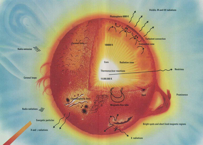
According to standard solar models, the solar structure looks like the following. The Sun is a sphere of solar radius R* = 6.96^10^{10} centimeters, initially composed by mass of about 70% hydrogen, 28% helium and 2% heavier elements. [Harvey, 1995, pp. 32]. About half of the mass and 98% of the energy generation (where hydrogen fuses into helium) exists in a core with a radius of about 0.25xR*. On top of the core is a stable region called the "radiative zone," where the energy is transported by radiation. At a solar radius of 0.713xR* and upwards to near the solar surface, the temperature is low enough that convection is the dominant mechanism for transporting energy. This zone is called the "convection zone."
Since each oscillation mode is sensitive to the solar interior's physical conditions where the amplitudes of the mode are the greatest, identifying oscillation modes is the mainstay of the helioseismologist's work.
Velocity Pictures of the Sun
To identify the oscillation modes, many helioseismology experiments start with a velocity picture of the Sun, where each pixel tracks the velocity of a small area on the solar surface by fixing on the Doppler shift of a spectrum line. One needs sequences of these images in order to identify oscillation modes.
Decomposing Doppler shift images into spatial spherical harmonics is the next step in identifying oscillation modes. [Harvey, J. 1995, pp. 35]. The coefficients of each spherical harmonic, as a function of time, are then Fourier transformed to generate a power spectrum as a function of three variables: nu, the frequency, the spherical harmonic degree l, and azimuthal order m. "L-nu figures" are a familiar diagram to helioseismologists- it is by using datasets like this, that oscillation modes are identified.
Inverse Problems
Inverse problems usually start with some precedure for predicting the response of a physical system with known parameters. Then we ask: how can we determine the unknown parameters from observed data? The goal of solving an inverse problem in helioseismology is to invert the observed data in order to derive the internal properties of the Sun. In other words, regard the density, temperature, sound speed (c), etc. as the unknown quantities and use the observed oscillation frequencies to obtain those unknowns.The SOHO/SOI-MDI group have obtained results for sound speed, rotation rate rate and pinning down the position of the hypothetical dynamo through inversions of measured frequency data.
Time-Distance Methods
The most common observation made in Earth seismology is that of the arrival time of the initial onset of the disturbance. If we know the variation of seismic velocity with depth within the earth, then we can calculate the travel time of rays between an earthquake and a receiver using geometrical approximations. So in principle, we can locate any earthquake in both time and space by by recording the arrival times of waves at stations worldwide.In time-distance helioseismology, the idea is the similar. One picks a point on the solar surface as the "source", and then assumes an annulus at some great circle around the point as a destination to which a wave may have travelled. Correlations between all points in the annulus are calculated, pulses with energy show in the calculated correlation function, and then one can derive time and distance for waves flowing in different directions.
The SOHO/SOI-MDI group have obtained results for sub-surface flows and other horizontal flows using time-distance methods and inversion methods.
More About Helioseismology
For a very nice helioseismology overview written by the GONG Project, see:For a very nice helioseismology tour written at Aarhus University, Denmark, see:
Technical paper by J. Christensen-Dalsgaard. Abstract, with link to full text (PDF):
More recent paper by M. P. Di Mauro. Abstract, with link to full text (PDF):
Seminar Presentation by P.B. Stark (UC Berkeley):
and Jørgen Christensen-Dalsgaard's (Aarhus University, Denmark) Lecture Notes:
If you wish to read some of the literature that introduces the newcomer to helioseismology, see:
General Info | Science Objectives & Proposals | Results, Images, & Documentation | Data Services & Info | Operations | Solar Center
Created by Amara Graps
Last Modified by PAK on February 19, 2009.